XYZLut & Destaggering¶

Once you have acquired a LidarFrame object, from a FrameSetSource as shown in the consumption section, you can perform numerous processing tasks.

As a reminder, the LidarFrame class batches lidar packets by full rotations into accessible fields of the appropriate type.

The LidarFrame object holds data in 2D fields (like RANGE, SIGNAL, REFLECTIVITY), and the SDK provides utilities to:

Project 2D fields into 3D point clouds.
Re-format 2D data for visualization and computer vision tasks.
Filter, mask, and modify frame data.

Sample recordings are available from the datasets listed at sample-data-download.

Projecting to 3D (Point Clouds)¶

The most common processing task is converting the 2D RANGE field into a 3D point cloud (XYZ points). The SDK performs this efficiently using a pre-computed Look-Up Table (LUT).

Common Setup

Python

View on GitHub ¶

# Other imports
# Other imports
# Other imports
from ouster.sdk import core

C++

View on GitHub ¶

#include "ouster/core/lidar_frame.h"
#include "ouster/core/typedefs.h"
#include "ouster/core/xyzlut.h"
using namespace ouster::sdk;

To convert 2D lidar data into a 3D point cloud,

you first create a reusable lookup table (XYZLut) from your sensor’s metadata. This table stores the 3D direction for every pixel. Then this table is applied to your 2D range image using the cartesian function, which efficiently calculates the final 3D (x, y, z) coordinates for every point.

The process involves two steps:

Build the lookup once: run XYZLut with your SensorInfo; it precomputes the per-pixel direction vectors.
Reuse it for every frame: feed the LUT and a RANGE field into cartesian (C++) or call the Python LUT object; it multiplies each range value by its direction vector and returns the XYZ coordinates (Eigen::Matrix in C++, (H, W, 3) array in Python).

For guidance on loading SensorInfo metadata when replaying a PCAP file, see the Obtaining Sensor Info. Once you have the sensor info, you are ready to create the XYZ look up table:

Python

View on GitHub ¶

# source = sensor.SensorFrameSetSource(sensor_hostname)
# sensor_info = source.sensor_info[0]
# frame = next(iter(source))[0]
xyzlut = core.XYZLut(sensor_info)
range = frame.field(core.ChanField.RANGE)
cloud = xyzlut(range)

C++

View on GitHub ¶

// sensor::SensorFrameSetSource source(sensor_hostname);
// auto sensor_info = source.sensor_info()[0];
// auto frame = LidarFrame(sensor_info);
auto xyzlut = core::XYZLut(info, /*use_extrinsics=*/ false);
auto range = frame.field(core::ChanField::RANGE);
auto cloud = xyzlut(range);

Now, you have your x, y, and z values, you can plot them easily to get something like:

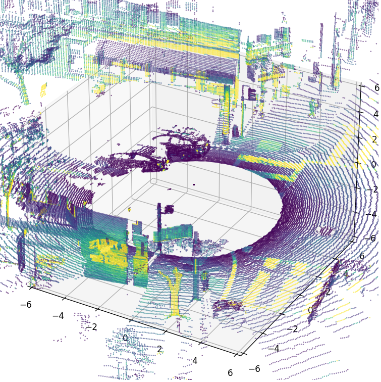
../../_images/lidar_frame_xyz_84.png — Point cloud from OS1 sample data (frame 84). Points colored by `SIGNAL` value.¶

You can find the complete code by clicking on the github icon on the code snippet or on our GitHub repository .

For a fast way to use a sensor to run XYZLut and visualize a similar image, refer to the pre-built Python example included in the SDK. Follow the instructions in the Python LidarFrame examples section.

Using Sensor Extrinsics in the LUT¶

use_extrinsics=True tells XYZLut to apply sensor_info.sensor_to_body with sensor_info.lidar_to_sensor_transform and use that combined 4×4 transform when building the lookup table (i.e., the LUT outputs points in the extrinsics frame rather than the sensor frame). The sensor_info.sensor_to_body matrix still comes straight from the sensor metadata and defaults to the identity matrix if the JSON omits it.

Python

View on GitHub ¶

lut_with_extrinsics = core.XYZLut(sensor_info, use_extrinsics=True)
return lut_with_extrinsics(frame)

C++

View on GitHub ¶

auto xyzlut = core::XYZLut(info, /*use_extrinsics=*/true);
auto cloud_in_extrinsics_frame = xyzlut(frame);

Applying External Transforms to the LUT¶

Users may find that they wish to apply an extra transform while projecting to Cartesian coordinates. Such a transform, likely an extrinsics matrix of some sort, can be baked directly into XYZLut constructor, which internally uses the make_xyz_lut function. This is more efficient than transforming every point cloud after projection.

In the following code, transform represents the external transformation matrix:

Python

View on GitHub ¶

# Custom pose: flip Z/Y and translate up 20 m and 1.5 m along X.
transform = np.eye(4, dtype=np.float64)
transform[2, 2] = -1.0
transform[1, 1] = -1.0
transform[2, 3] = 20000.0  # millimetres (20 m)
transform[0, 3] = 1500.0   # millimetres (1.5 m)
# Compose it with the sensor’s existing lidar→sensor transform
adjusted = deepcopy(sensor_info)
adjusted.lidar_to_sensor_transform = transform @ sensor_info.lidar_to_sensor_transform

# Build the LUT from the modified metadata and project the frame.
xyzlut = core.XYZLut(adjusted, use_extrinsics=False)
cloud_adjusted = xyzlut(frame)
return cloud_adjusted

C++

View on GitHub ¶

// Custom pose: flip Z/Y and translate up 20 m and 1.5 m along X.
core::mat4d transform = core::mat4d::Identity();
transform(2, 2) = -1.0;
transform(1, 1) = -1.0;
transform(2, 3) = 20000.0;  // millimetres
transform(0, 3) = 1500.0;   // millimetres
// Compose with the existing lidar_to_sensor transform.
core::SensorInfo adjusted = info;
core::mat4d combined = transform * info.lidar_to_sensor_transform;

// Override the transform before building the LUT.
adjusted.lidar_to_sensor_transform = combined;

core::XYZLut lut_adjusted(adjusted, /*use_extrinsics=*/false);
auto cloud_adjusted = lut_adjusted(frame);
return cloud_adjusted;

Using the use_extrinsics=False returns the sensor-frame directions/offsets with no extra transform. Hence, to apply external transform, we retrieve the SensorInfo, multiply in their custom 4×4 matrix, and then build the LUT—so the LUT bakes in the pose we supplied instead of applying it afterward.

NOTE The SDK also provides a :py:class::ouster.sdk.core.XYZLutFloat in Python, which can be used when one needs to save memory or work in float32.

2D Data Layout: Staggered vs. Destaggered¶

The default representation of LidarFrame stores data in staggered columns, meaning that each column contains measurements taken at a single timestamp. As the lasers flashing at each timestamp are arranged over several different azimuths, the resulting 2D image if directly visualized is not a natural image.

Let’s take a look at a typical staggered representation:

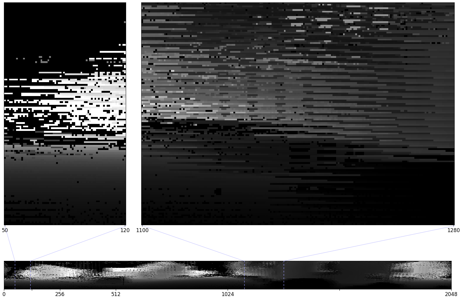
../../_images/lidar_frame_staggered.png — LidarFrame `RANGE` field visualized with `matplotlib.pyplot.imshow()` and simple gray color mapping for better look.¶

To re-format the data into a natural 2D image representation, you must destagger it. We destagger the relevant field of the LidarFrame with destagger (destagger(), core.destagger() function):

Destaggering re-orders the columns to correspond to their azimuth angle instead of timestamps. This is essential for 2D visualization and many 2D computer vision algorithms.

The API accepts an optional inverse flag - set it to true when you need to undo a previous destagger by reapplying the per-row pixel shifts and return data to the original staggered layout.

Python

View on GitHub ¶

"""Get staggered and destaggered reflectivity images."""

reflectivity = frame.field(core.ChanField.REFLECTIVITY)
reflectivity_destaggered = core.destagger(sensor_info, reflectivity)

C++

View on GitHub ¶

std::cout << "\n3. Getting staggered and destaggered images of Reflectivity..." << std::endl;

auto reflectivity = frame.field(core::ChanField::REFLECTIVITY);
auto reflectivity_destaggered = core::destagger(info, reflectivity, false);

After destaggering, the 2D image makes visual sense.

Python: Plot destaggered reflectivity image

To generate staggered and destaggered images yourself, you can try the following sample code:

View on GitHub ¶

import sys
from pathlib import Path

import matplotlib.pyplot as plt
import numpy as np
from more_itertools import nth

# [doc-stag-core-frames]
from ouster.sdk import core, pcap

if len(sys.argv) < 2:
    raise SystemExit("Usage: python viz.py <pcap_path>")

pcap_path = str(Path(sys.argv[1]).expanduser())
# open a FrameSetSource directly from the PCAP/metadata pair
source = pcap.PcapFrameSetSource(pcap_path)
metadata = source.sensor_info[0]
# pull the 84th frame set (adjust the index for your dataset)
frame_set = nth(source, 84)
if frame_set is None:
    raise RuntimeError("Expected at least 85 frame sets in source")
# single-sensor PCAP; take the first LidarFrame
frame = frame_set[0]
if frame is None:
    raise RuntimeError("Expected a LidarFrame at sensor index 0")
# reflectivity in the default staggered layout
reflectivity = frame.field(core.ChanField.REFLECTIVITY).astype(np.uint32)
# destagger using the metadata intrinsics
reflectivity_destaggered = core.destagger(metadata, reflectivity)
# [doc-etag-core-frames]
plt.imshow(reflectivity_destaggered, cmap='gray', resample=False)
plt.show()

The above code gives the scene below (see the long strip at the bottom). We’ve magnified two patches for better visibility atop.

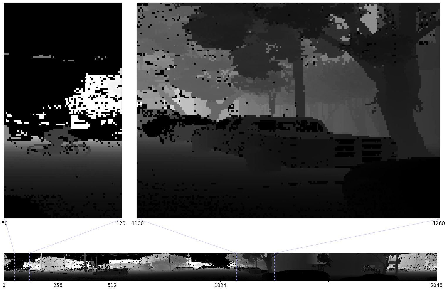
../../_images/lidar_frame_destaggered.png — **destaggered** LidarFrame `RANGE` field¶

After destaggering, we can see the scene contains a man on a bicycle, a few cars, and many trees. This image now makes visual sense, and we can easily use this data in common visual task pipelines.

Reshaping XYZ to 2D¶

Users may find that they wish to access the x, y, and z coordinates of a single return in a similar way. As the conversion to Cartesian coordinates returns an Eigen::Array n x 3, with n = w * h, reshaping the resulting array is necessary.

We can combine our knowledge in projecting into Cartesian coordinates and destaggering using the following function:

Python

View on GitHub ¶

def get_x_in_image_form(frame: core.LidarFrame,
                        sensor_info: core.SensorInfo,
                        destaggered: bool = False):
    """Return the destaggered X coordinate image."""
    h = sensor_info.format.pixels_per_column
    w = sensor_info.format.columns_per_frame

    # Get the XYZ in (H, W, 3) numpy array form
    xyzlut = core.XYZLut(sensor_info, use_extrinsics=False)
    xyz = xyzlut(frame)

    # Extract X coordinate (equivalent to cloud.col(0) in C++)
    x_image = xyz[:, :, 0].reshape(h, w)
    # Apply destagger if desired
    if not destaggered:
        return x_image

    x_destaggered = core.destagger(sensor_info, x_image)
    return x_destaggered

C++

View on GitHub ¶

core::img_t<double> get_x_in_image_form(const core::LidarFrame& frame,
                                        const core::SensorInfo& info,
                                        bool destaggered = false) {
    // For convenience, save w and h to variables
    const size_t w = info.format.columns_per_frame;
    const size_t h = info.format.pixels_per_column;

    // Get the XYZ in ouster::Points (n x 3 Eigen array) form
    core::XYZLut xyzlut(info, /*use_extrinsics=*/ false);
    auto cloud = xyzlut(frame);

    // Access x and reshape as needed, not that the values in cloud.col(0) are ordered
    auto x_image = Eigen::Map<const core::img_t<double>>(cloud.col(0).data(), h, w);
    // Apply destagger if desired
    if (!destaggered) {
        return x_image;
    }
    auto x_destaggered = core::destagger<double>(x_image, info.format.pixel_shift_by_row);
    return x_destaggered;
}

This demonstrates the functionality with x, but it can be easily expanded to cover y and z as well.

Populating LidarFrames¶

This reference has covered how to access, project, and destagger LidarFrame contents. But in order for LidarFrames to be useful, we need a way to populate them with packet data!

For convenience, the Ouster Python SDK provides batching helpers for both live and recorded data.

See the data consumption section for more information.

Adding custom fields to a LidarFrame¶

It’s possible to add custom fields to a LidarFrame. This is especially useful if you want to add custom data to an OSF file for visualization purposes.

You can find more information about this in the documentation Adding custom fields to a LidarFrame.

XYZLut & Destaggering¶

Projecting to 3D (Point Clouds)¶

Using Sensor Extrinsics in the LUT¶

Applying External Transforms to the LUT¶

2D Data Layout: Staggered vs. Destaggered¶

Reshaping XYZ to 2D¶

Correlating 2D and 3D Data¶

Populating LidarFrames¶

Adding custom fields to a LidarFrame¶