

Visualizations in 3D
The Ouster Python SDK provides two visualization utilities for user convenience. These are introduced briefly below.
Visualization with Open3d
The Open3d library contains Python bindings for a variety of tools for working with point cloud
data. Loading data into Open3d is just a matter of reshaping the numpy representation of a point
cloud, as demonstrated in the examples.pcap.pcap_3d_one_frame() example:
# compute point cloud using core.SensorInfo and core.LidarFrame
xyz = core.XYZLut(metadata)(frame)
Once you have the xyz numpy array, you can create an Open3d point cloud and visualize it as follows:
# create point cloud and coordinate axes geometries
cloud = o3d.geometry.PointCloud(
    o3d.utility.Vector3dVector(xyz.reshape((-1, 3))))  # type: ignore
axes = o3d.geometry.TriangleMesh.create_coordinate_frame(
    1.0)  # type: ignore

# initialize visualizer and rendering options
vis = o3d.visualization.Visualizer()  # type: ignore

vis.create_window()
vis.add_geometry(cloud)
vis.add_geometry(axes)
ropt = vis.get_render_option()
ropt.point_size = 1.0
ropt.background_color = np.asarray([0, 0, 0])

# initialize camera settings
ctr = vis.get_view_control()
ctr.set_zoom(0.1)
ctr.set_lookat([0, 0, 0])
ctr.set_up([1, 0, 0])

# run visualizer main loop
print("Press Q or Escape to exit")
vis.run()
vis.destroy_window()
source.close()
The examples.open3d module contains a more fully-featured visualizer built using the Open3d
library, which can be used to replay pcap files or visualize a running sensor. The bulk of the
visualizer is implemented in the examples.open3d.viewer_3d() function.
Note
You’ll have to install the Open3d package from PyPI to run this example.
As an example, you can view frame 84 from the sample data by running the following command:
$ python3 -m ouster.sdk.examples.open3d_example --pcap $SAMPLE_DATA_PCAP_PATH --start 84 --pause
PS > py -3 -m ouster.sdk.examples.open3d_example –pcap $SAMPLE_DATA_PCAP_PATH –start 84 –pause
You may also want to try the --sensor option to display the output of a running sensor. Use the
-h flag to see a full list of command line options and flags.
Running the example above should open a window displaying a scene from a city intersection, reproduced below:
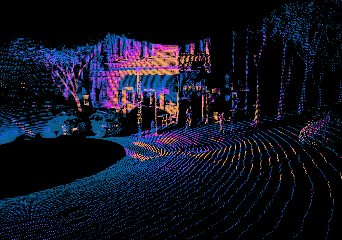
Open3D visualization of OS1 sample data (frame 84). Points colored by SIGNAL field.
You should be able to click and drag the mouse to look around. You can zoom in and out using the mouse wheel, and hold control or shift while dragging to pan and roll, respectively.
Hitting the spacebar will start playing back the rest of the pcap in real time. Note that reasonable performance for real-time playback requires relatively fast hardware, since Open3d runs all rendering and processing in a single thread.
All of the visualizer controls can be viewed on the terminal by pressing ? while the visualizer
window is in focus.
Visualization with Matplotlib
You should have defined source using either a pcap file or UDP data streaming directly from a
sensor, please refer to Quickstart Guide for introduction.
Note
Below pictures were rendered using OS2 128 Rev 05 Bridge sample data.
Let’s read from source until we get to the 50th frame of data:
from more_itertools import nth
frame_set = nth(source, 50)
frame = frame_set[0]
Note
If you’re using a sensor and it takes a few seconds, don’t be alarmed! It has to get to the 50th frame of data, which would be 5.0 seconds for a sensor running in 1024x10 mode.
We can extract the range measurements from the frame of data stored in the core.LidarFrame
datatype and plot a range image where each column corresponds to a single azimuth angle:
range_field = frame.field(core.ChanField.RANGE)
range_img = core.destagger(sensor_info, range_field)
We can plot the results using standard Python tools that work with numpy data types. Here, we extract a column segment of the range data and display the result:
import matplotlib.pyplot as plt
plt.imshow(range_img[:, 640:1024], resample=False)
plt.axis('off')
plt.show()
Note
If running plt.show gives you an error about your Matplotlib backend, you will need a GUI
backend such as TkAgg or Qt5Agg in order to visualize your data with matplotlib.
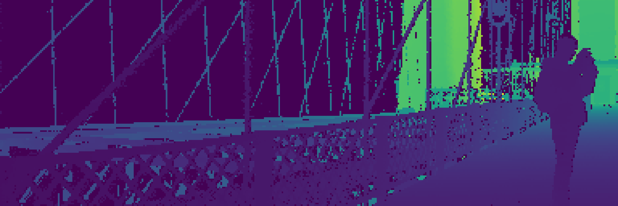
Range image of OS2 bridge data. Data taken at Brooklyn Bridge, NYC.
In addition to viewing the data in 2D, we can also plot the results in 3D by projecting the range measurements into Cartesian coordinates. To do this, we first create a lookup table, then use it to produce X, Y, Z coordinates from our frame data with shape (H x W x 3):
xyzlut = core.XYZLut(sensor_info)
xyz = xyzlut(frame)
Now we rearrange the resulting numpy array into a shape that’s suitable for plotting:
import numpy as np
[x, y, z] = [c.flatten() for c in np.dsplit(xyz, 3)]
ax = plt.axes(projection='3d')
r = 10
ax.set_xlim3d([-r, r])
ax.set_ylim3d([-r, r])
ax.set_zlim3d([-r/2, r/2])
plt.axis('off')
z_col = np.minimum(np.absolute(z), 5)
ax.scatter(x, y, z, c=z_col, s=0.2)
plt.show()
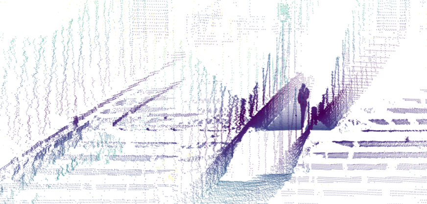
Point cloud from OS2 bridge data with colormap on z. Data taken at Brooklyn Bridge, NYC.
You should be able to rotate the resulting scene to view it from different angles.
To learn more about manipulating lidar data, see:
Set coloring mode or image mode using LidarFrameViz API
From 0.15.0, you can now set an image mode or coloring mode using visualization api.
from ouster.sdk import viz, open_source
import sys

src = open_source(sys.argv[1])

sviz = None
def iter():
    global sviz
    for frame_set in src:
        sviz._frame_viz.update(frame_set)
        break
    sviz._frame_viz.select_cloud_mode("RANGE")
    sviz._frame_viz.select_img_mode(0, "RANGE")
    for frame_set in src:
        yield frame_set

sviz = viz.SimpleViz(src.sensor_info)
sviz.run(iter())